TAMU/UCSD/GT Seedling Profile (BIRDSHOT)#
Batch-wise Improvement in Reduced Design Space using a Holistic Optimization Technique
Note
This profile is still under development. The information provided in this profile is based on [Arroyave22, BIRDSHOT22] and interviews with BIRDSHOT team members.
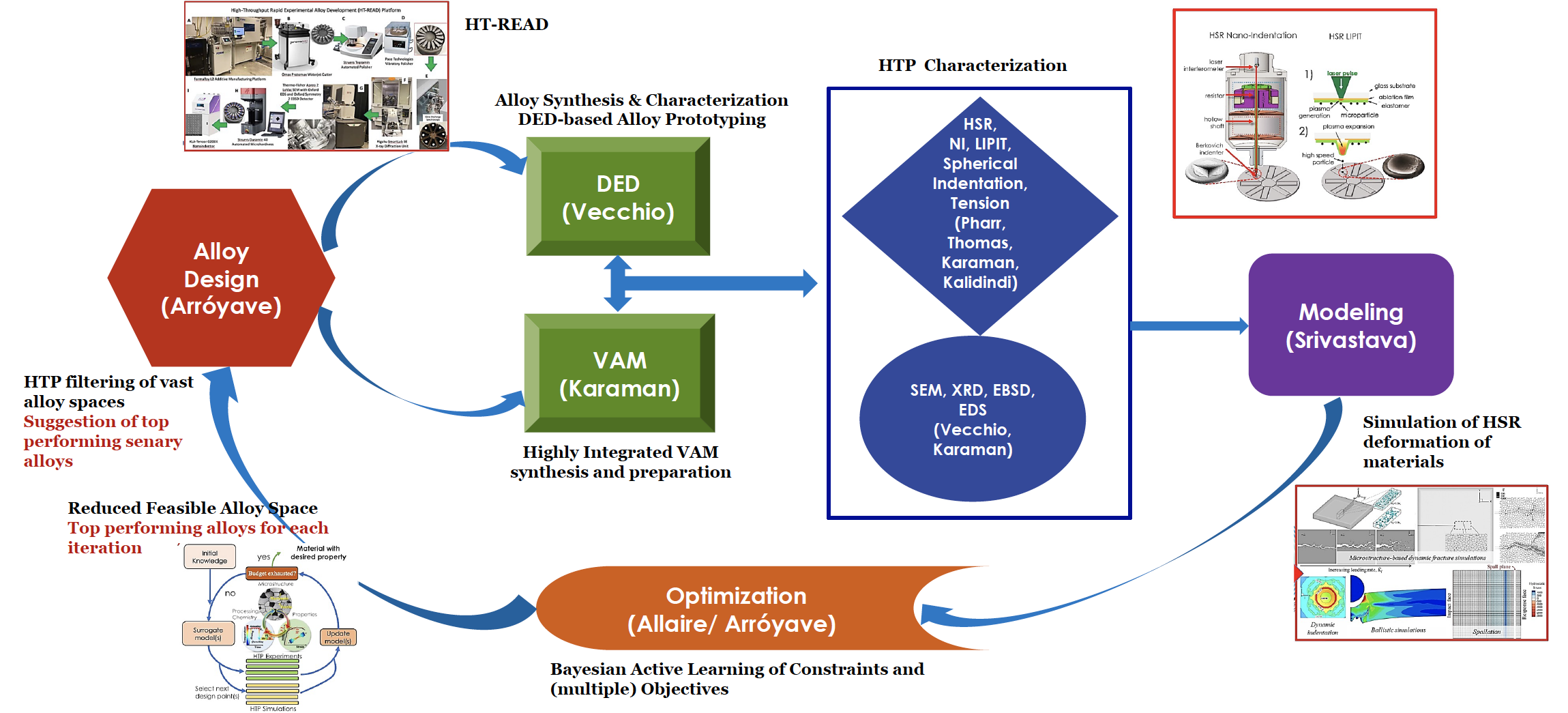
Fig. 14 Overview of the BIRDSHOT collaborative workflow#
Collaboration#
The BIRDSHOT seedling is a collaboration between eight different teams from four institutions. The collaborative workflow is illustrated in Fig. 14. This is an iterative process.
Alloy search and design
High-throughput design [Arróyave, TAMU]
Processing:
Vacuum arc melting (VAM) [Karaman, TAMU]
Directed energy deposition (DED) [Vecchio, UCSD]
Characterization:
Tension [Karaman, TAMU]
High strain rate nanoindentation (HSR-NI) [Pharr, TAMU]
Laser induced projectile impact testing (LIPIT) [Thomas, TAMU]
Spherical indentation [Kalidindi, GT]
Data-driven models [Srivastava, TAMU]
Optimization [Allaire, TAMU]
Data management#
The BIRDSHOT seedling uses a shared filesystem approach for data management via Google Drive. Information is organized according to a well-defined filesystem hierarchy and naming conventions. The team is working with Contextualize to automate curation, collection and analysis workflows.
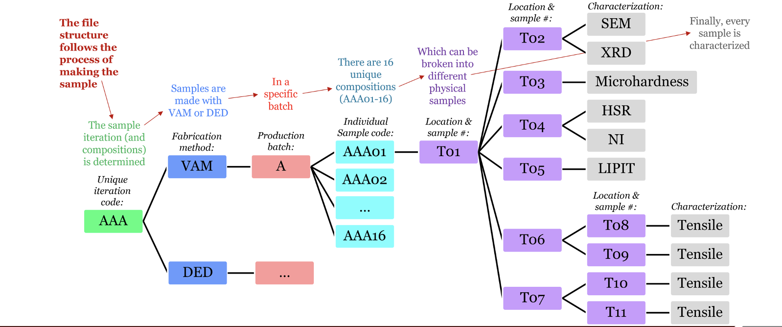
Fig. 15 Filesystem organization and naming conventions (VAM)#
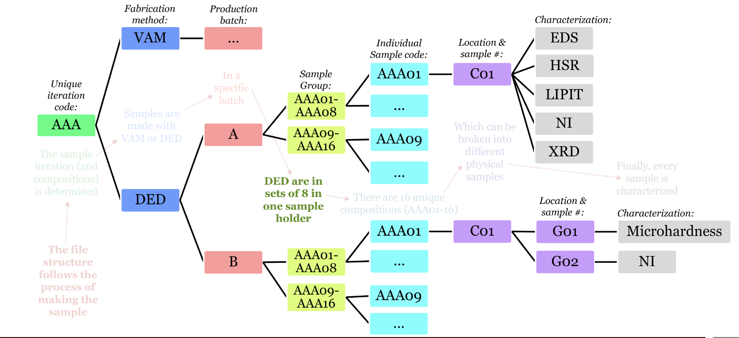
Fig. 16 Filesystem organization and naming conventions (DED)#
Unique code: AAA, AAB, AAC
Fabrication method: VAM, DED
Production batch:
01-n (VAM is single sample, DED is 8 samples on a single sample holder) Location and sample number:
Process: HSR, NI, LIPIT, Spherical indentation, tension, SEM, XRD, EBSD, EDS
Data summary#
Data is organized in the shared folder under three primary folders. Below is a summary of data types in each folder:
/data/:NI: nmd, nmdproj, txt
SEM: tiff
Carta: json
Other: xlsx
/FeCoCrNiV - Synthesis Sub ProjectEDS/EBSD: bmp, dat, tiff
XRD: hdf5, rasx, scn
BBO: m, mat
Other: csv, png, pptx, py, xslx
/Sample Data:EDS/EBSD: dat, tiff
XRD: bmp, par, raw, scn
BBO: m, mat
Other: csv, pdf, png, ppty, py, tra, txt, xslx
Compiled results and summary tables are generally provided in Excel spreadsheets, however work is being done with the Contextualize data seedling to use custom web-based forms with JSON output stored in the same folder structure. Other types of research assets are present (NI, XRD, EBSD data; source code), but according team members, many research assets are maintained by individual labs or researchers and only summary results shared in Drive.
Alloy search and design#
The alloy search and design process centers on BO for the compositional space. The basic workflow is as follows:
Candidate alloys are sent to the team from the two processing routes (VAM or DED) with production job travelers. Each iteration has a unique sample identifier.
Preliminary characterization
For each iteration, summary results are provided in Excel to BO team
Bayesian optimization (Matlab)
Objectives: hardness, ultimate tensile strength/yield strength (UTS/YS), strain rate sensitivity
60 experiments per iteration, 3 objectives, executed on TAMU supercompute.
8 samples each from Low and High stacking fault energy (SFE)
Original runtime of 42 hours with 400 cores has been reduced to ~1 hour
Alloy search across constrained compositional space
Synthesis and bulk property characterization#
Target property data informs materials design
Batch material production
Thermomechanical processing
Microstructural property characterization
Microstructure and homogeneity evaluation (XRD)
Chemical analysis (EDS)
Mechanical property characterization
Microhardness
Tension
Rapid experimental alloy development#
High throughput characterization#
Nanoindendation#
Workflow:
Receive samples from fabrication team
Obtain elastic modulus and preliminary hardness
High strain rate testing using HSR nanoindenter
Optical profiling of indents to determine degree of pile-up or sing-in
Pile-up/sink-in correction
Submit data to computational team and deliver samples to LIPIT group
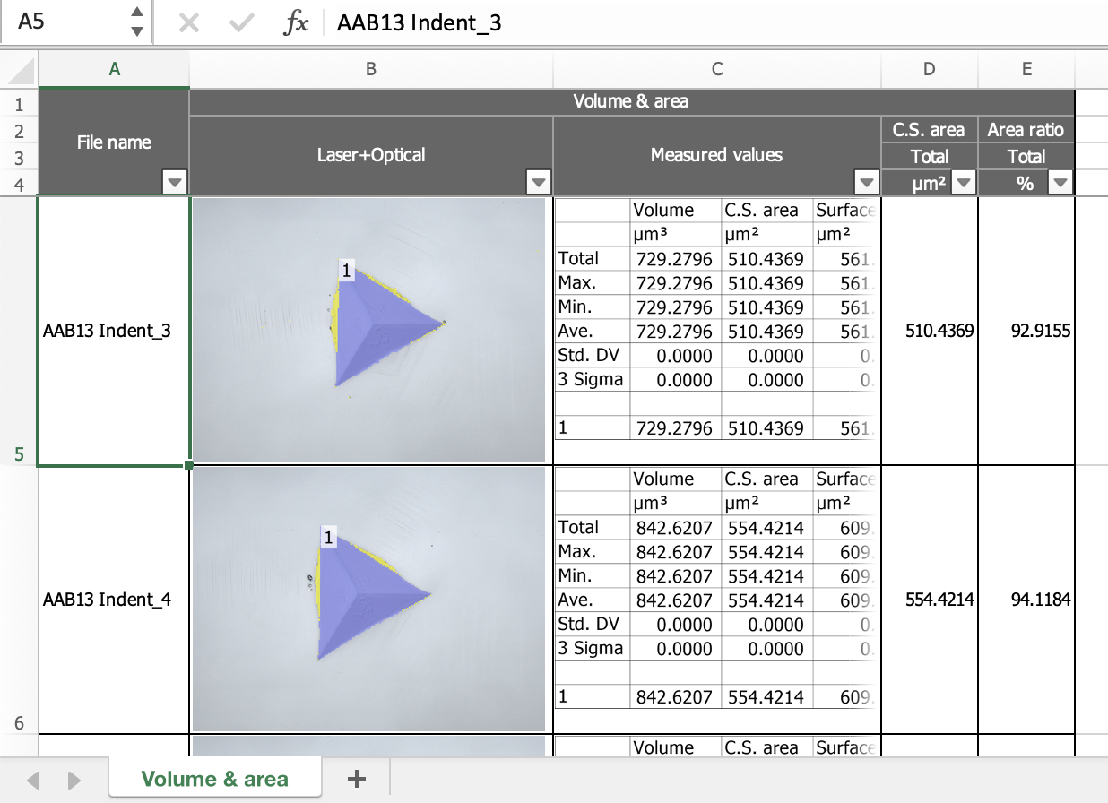
Fig. 17 Example spreadsheet with NI optical profiles#
As illustrated in Fig. 17, NI visualizations are included in summary spreadsheets.